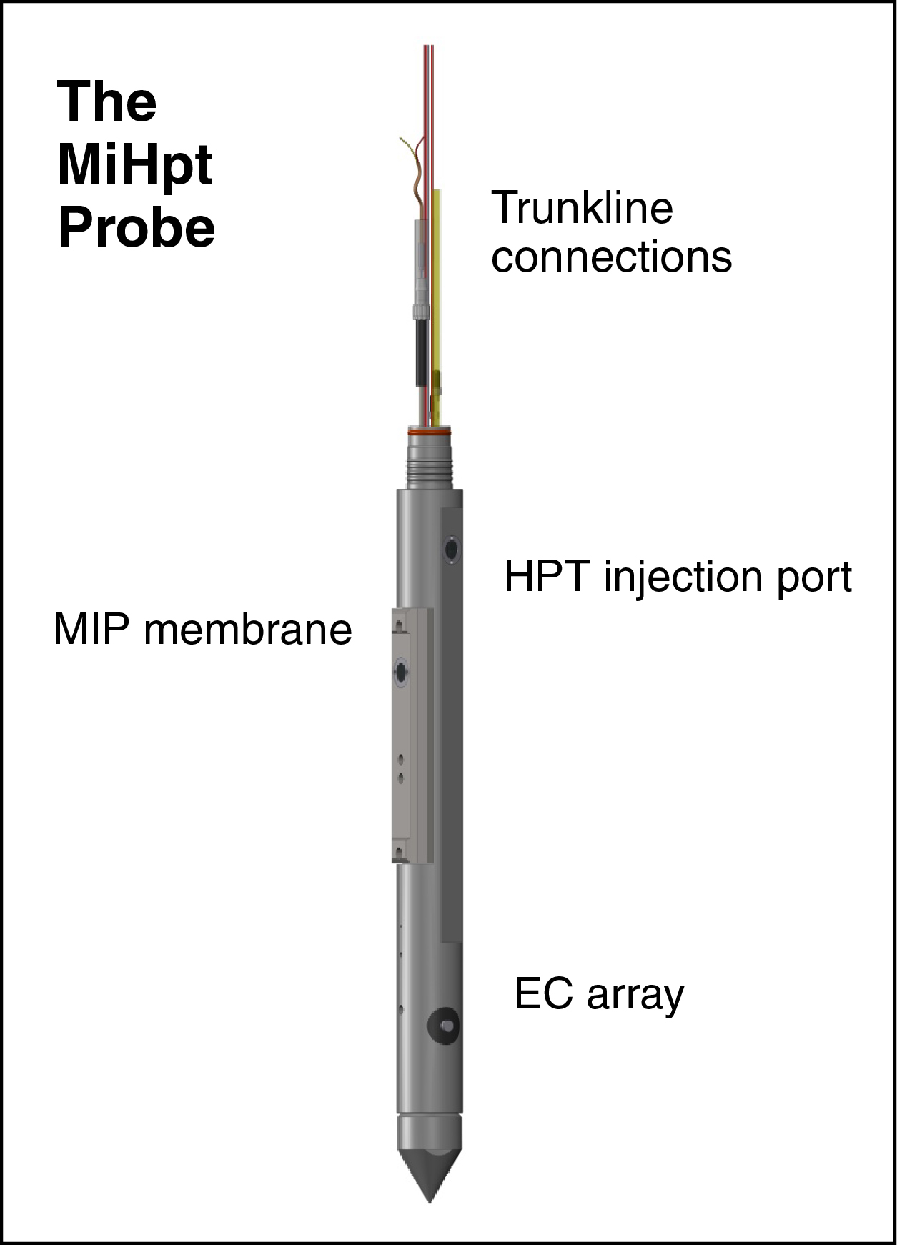
The combined membrane interface probe (MIP) and hydraulic profiling tool (HPT) is designated as the MiHpt probe (Figure G-1). The MIP part of the system includes the downhole probe with semipermeable membrane, trunkline strung through the probe rods, and uphole gas chromatograph (GC); the GC typically includes a photoionization detector (PID), flame ionization detector (FID), and halogen specific detector (XSD). The HPT part of the system contains the screened port on the side of the probe, downhole pressure transducer, and uphole pump with flow meter and trunkline. The MiHpt probe includes an electrical conductivity (EC) array.
Figure G-1. Schematic of an MiHpt probe (combined MIP and HPT).
The semipermeable membrane on the side of the probe allows volatile organic compounds (VOCs) to pass from the soil into the clean carrier gas stream under a concentration gradient (Figure G-2). The nitrogen carrier gas sweeps the VOCs up the trunkline to the GC detectors at the surface. A heater block at the membrane is heated to about 100 degrees Celsius to enhance VOC migration from the soil across the membrane. The probe is advanced incrementally into the formation. Advancement is stopped for approximately 60 seconds at each 1 ft (30 cm) increment. This allows time for the VOCs to cross the membrane and be swept up to the GC detectors. A stringpot mounted on the mast of the direct-push machine tracks depth as the probe is advanced. The acquisition software plots the detector response at the correct depth on the computer screen as the log is being run.
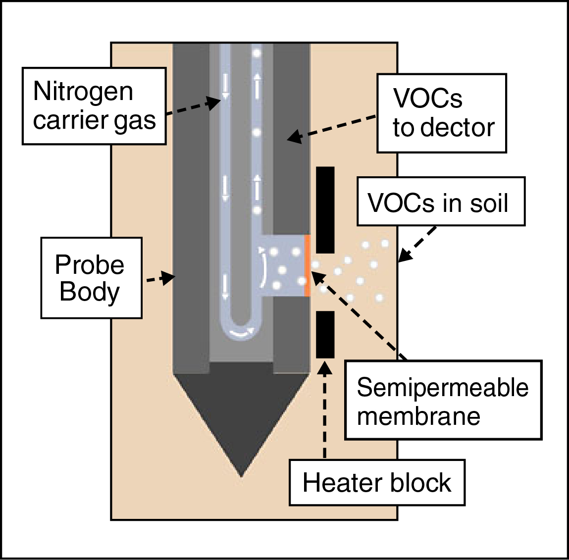
Figure G-2. Operating principles for the MiHpt probe.
In Figure G-3, a pump (B) at the surface pumps clean water down the trunkline and out the screened port (F) on the side of the probe into the unconsolidated formation. A flow meter (B) measures the injection flow rate. The downhole pressure sensor (E) measures the pressure required to inject water into the formation. The injection pressure and flow are plotted on screen vs. depth as the probe is advanced. An electrical conductivity array (G) also provides an EC log of the formation.
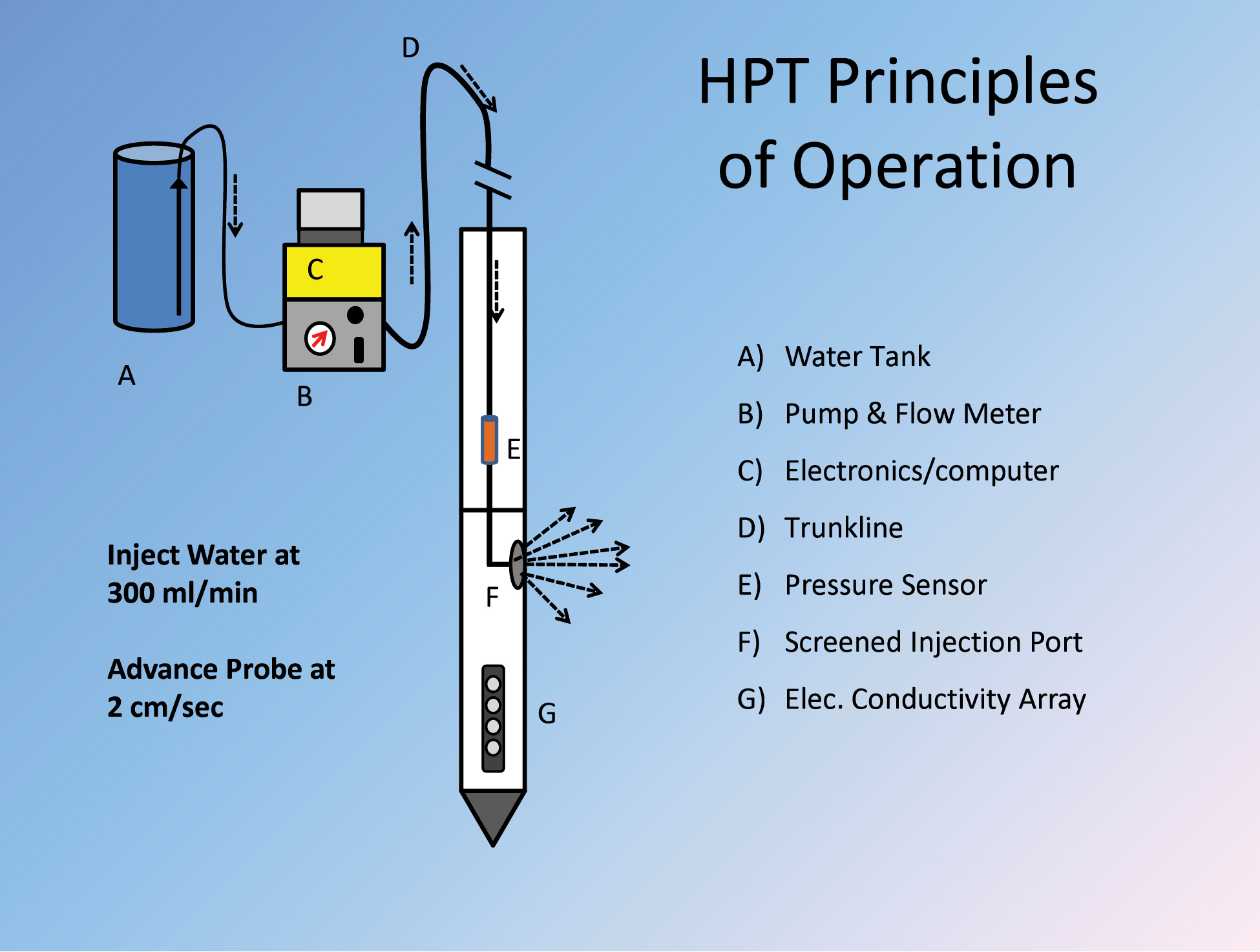
Figure G-3. HTP operation.
MiHpt log interpretation is relatively simple. On the EC and detector data log (Figure G-4) for Case Study 1—a tetrachloroethene (PCE)-contaminated site in Skuldelev, Denmark—the left graph plots the EC log vs. depth. In fresh water formations, low EC values generally indicate coarse-grained materials (sand and gravel), while higher EC values usually indicate elevated clay content. This EC log indicates primarily sand and gravel to a depth of about 7 m. The graph in the center plots the PID detector response vs. depth, and the graph on the right plots the XSD detector response vs. depth. Higher detector response indicates higher concentrations of contaminants.
The detector logs show that, above 3 m, there is little or no contamination, while the contaminant concentrations increase significantly at 3 m–6 m and then drop off again. The XSD is sensitive to chlorinated VOCs such as PCE and trichloroethene (TCE). The PID is sensitive to aromatic compounds like benzene and toluene, but also responds to the double bond present in the chlorinated ethenes (for example, PCE, TCE, and dichlorothene [DCE]). Thus, from the combined PID and XSD data, it can be inferred that the primary contaminants are chlorinated ethenes, although sampling is required to confirm this initial interpretation. The combined data from the EC log and detector responses indicate that the contaminants are primarily in the permeable and transmissive sand and gravel of the local formation.

Figure
After this log (Figure G-5) was completed, a direct-push, discrete-interval sampling tool was used to collect groundwater samples at targeted intervals based on the detector response log. Only 1 ft (30 cm) of screen was opened at each depth interval. The samples were analyzed at a fixed lab by gas chromatography/mass spectrometry for the typical suite of VOC contaminants. The results for PCE+TCE+DCE are plotted over the PID and XSD logs at the depths where they were collected (red triangles). Duplicate samples were collected in the field at a couple of intervals and those results are plotted with the original sample results. The PID and XSD detector logs correlate well with the groundwater sample results.
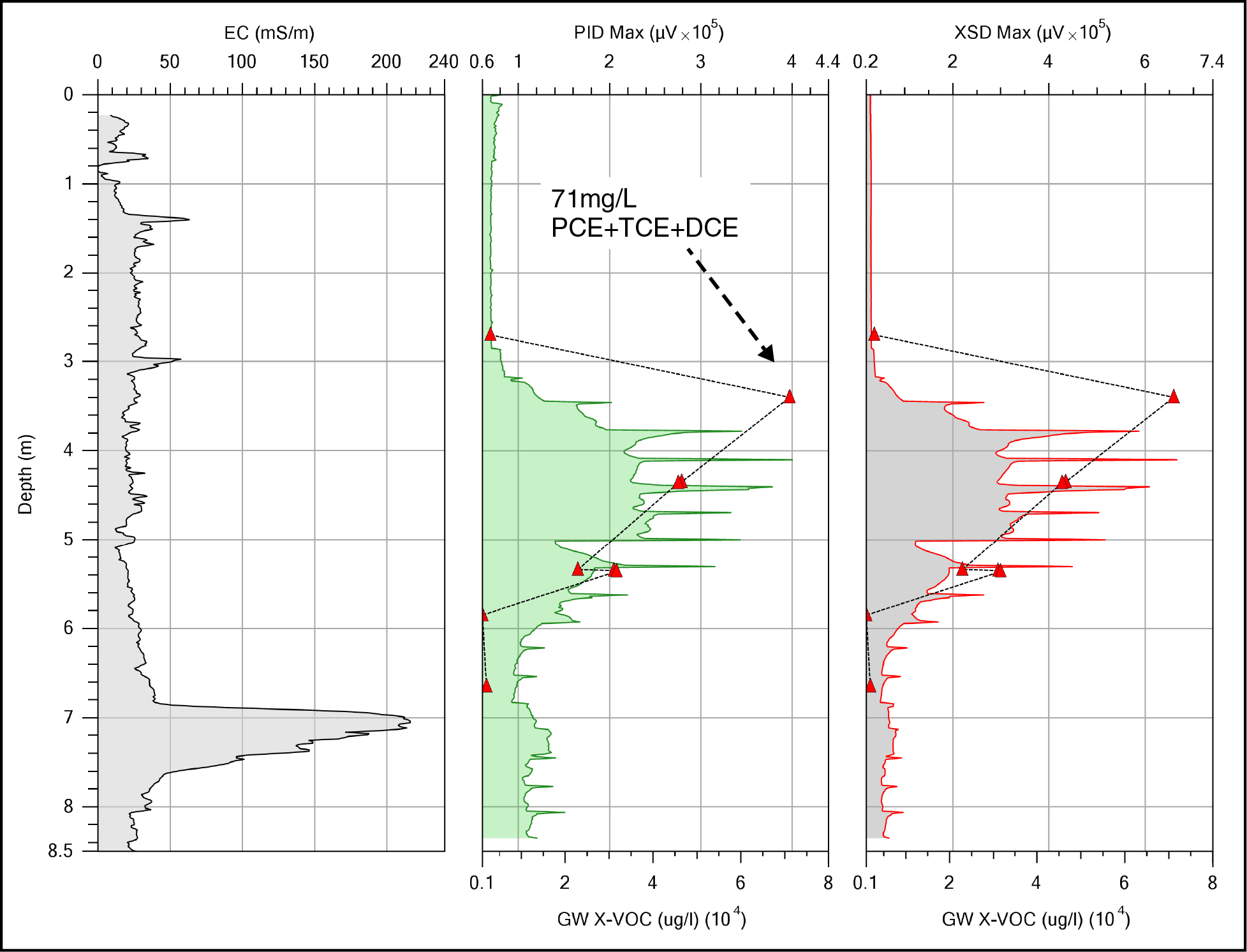
Figure G-5. SK05 MIP log data with groundwater X-VOC results.
For the HPT log data from the SK05 location (Figure G-6), the EC log is again plotted on the left, while the HPT pressure is in the center graph and the HPT flow rate is on the right; all are presented versus depth. For HPT logs, lower injection pressure indicates higher permeability and higher injection pressure indicates lower permeability. For this log, the pressure peak between the surface and the 1m depth indicates some fine-grained soils. This is followed by relatively low HPT pressure down to just above 7m, indicating a good permeability formation. Below 7m, the HPT pressure increases, indicating lower-permeability materials. The HPT flow rate is relatively constant down the log, with some flow decrease as the probe passes through the higher-pressure material below 7m. The slow rise in the HPT pressure from about 1m deep to just below 7m where the fine-grained material is penetrated indicates the increase in hydrostatic pressure (dashed line) as the probe advances below the water table. During this log probe, advancement was stopped at about 3m and 5m to run dissipation tests. The HPT injection flow was turned off and the ambient piezometric pressure was measured. With this information, the piezometric pressure line could be plotted and the local water level calculated.

Figure G-6. EC, pressure, and flow data for the SK05 MiHpt log.
Continuous soil cores were collected next to the SK05 location (Figure G-7). Photos of some of the core samples are shown next to the HPT pressure and flow rate logs. The cores from the upper 7m are composed mostly of sand and gravel with minor amounts of silt and clay. Below 7m, the core samples contain primarily fine-grained, silty clay with a little sand and occasional gravel sized clasts. It is thus evident that the HPT pressure data provide a good representation of the local lithology and formation permeability.

Figure G-7. SK05 HPT log data.
All of the MiHpt data from the SK05 location are combined in one log (Figure G-8). The HPT flow data (blue dash) are shown on the same graph as the HPT pressure data. The axis for the flow rate data is provided on the bottom of the graph. These data show that the chlorinated volatile organic compound (X-VOC) contamination at this location is present in the permeable formation materials and could readily migrate in the groundwater.
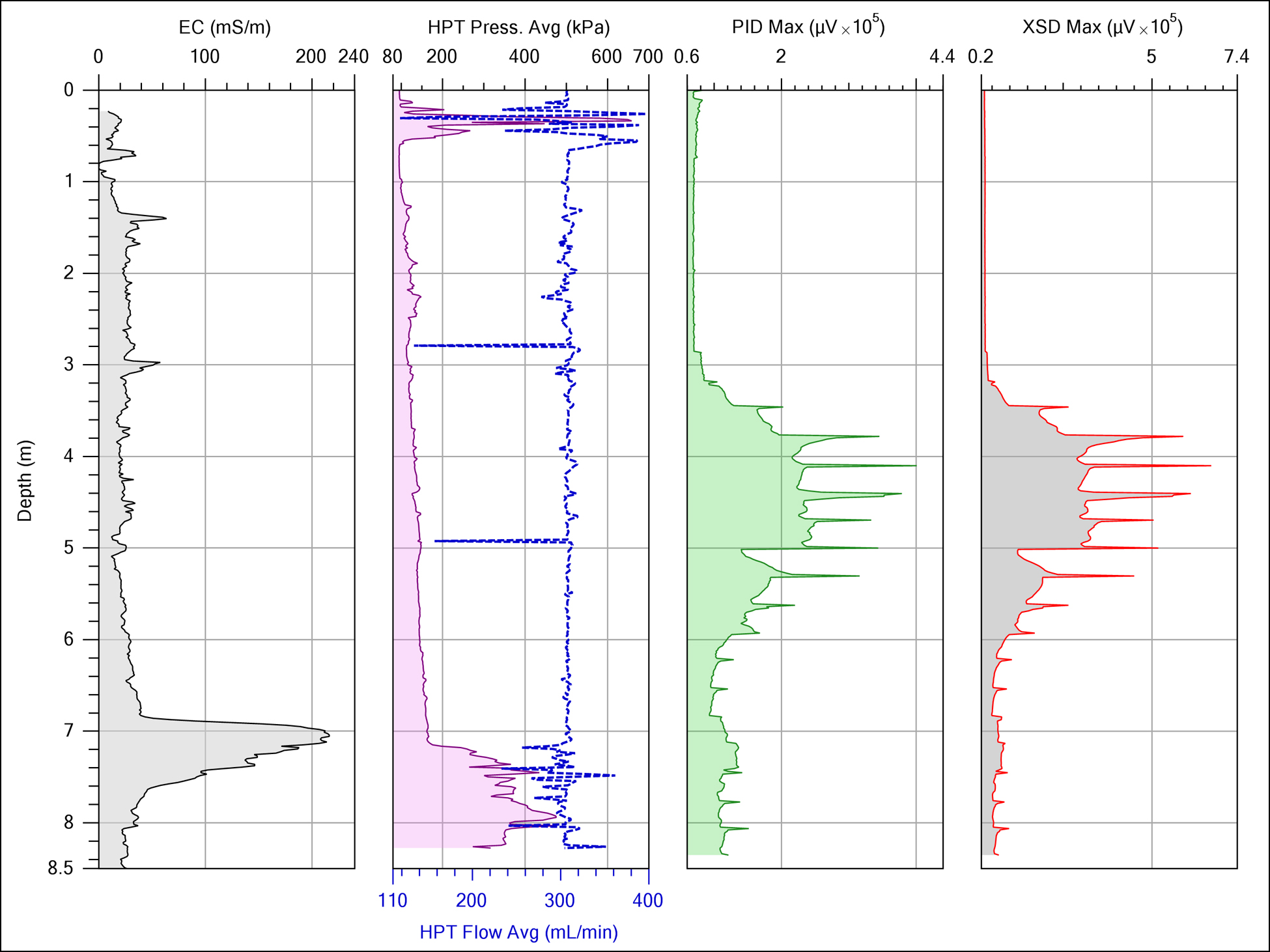
Figure G-8. Complete SK05 MiHpt log.
The small town of Skuldelev is located about an hour west of Copenhagen in the pastoral countryside of Denmark (Figure G-9). This region was glaciated and the town is underlain by glacial deposits and related sediments. A manufacturing facility located adjacent to the town’s community park used PCE as a cleaning solvent, and it was released to the environment (Figure G-10). Previous investigations had delineated at least three DNAPL hot spots and a groundwater plume extending more than a kilometer off site; however, the groundwater plume followed an irregular course, and the results of the earlier investigations did not determine the reason for this type of plume migration.
MiHpt logs were run in a transect across the site to study the contaminant distribution and evaluate the local hydrostratigraphy. The SK05 log is one of the logs along this transect (blue circle).

Figure G-9. Site location map, Skuldelev, Denmark.

Figure G-10. Skuldelev site map.
Figure G-11 provides a cross section of the HPT pressure logs, with perspective facing south. As shown, the increase in HPT pressure in each log corresponds to the top of the clay-till; thus, below this HPT pressure increase, the formation is primarily clay-till, and the lower HPT pressure above corresponds to the sand and gravel formation. The dashed line connecting the point where HPT pressure increases in each log provides an outline of the surface of the clay-till at depth. This cross section shows what appears to be a small valley cut into the clay-till, possibly by a late-post-glacial stream. Later, this small valley was filled with sand and gravel (glacial outwas

Figure G-11. Skuldelev HPT pressure cross section.
In Figure G-12, the HPT pressure logs (black lines) have been overlaid with the XSD detector logs (red with blue fill), indicating elevated XSD responses at the SK05 and SK07 logs near the center of the buried stream valley. Thus, it appears that the groundwater plume is migrating off site by following the migration pathway created by the buried stream valley. More than 10 years of investigative work had been conducted at this facility; however, not until completion of the MiHpt logs was the controlling factor for the groundwater plume migration understood.
On the west side of the cross section are very high XSD responses down in the clay-till, with little or no contamination in the overlying sand and gravel (Figure G-13).

Figure G-12. Skuldelev HPT pressure and XSD cross section.
By plotting the sewer lines on the site map (black dash) (Figure G-13), a sewer line junction is evident next to the SK12 log at the location of a DNAPL hot spot. An earlier investigation revealed that waste solvent (PCE) had been poured down the drain at the facility, and a leak in the sewer line junction next to the SK12 location led to development of this hot spot with DNAPL. Additionally, migration of PCE vapors through the sewer lines and in the sewer trenches led to vapor intrusion into several homes at the site. Several of the old sewer lines have been replaced and mitigation of the vapor intrusion is underway.
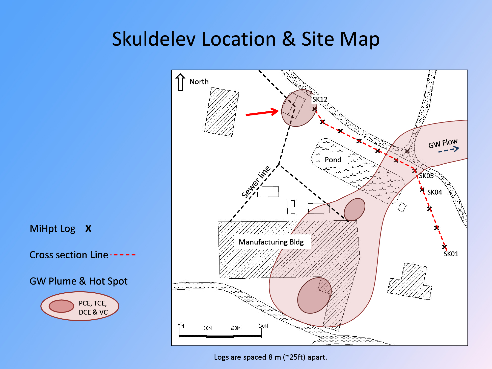
Figure G-13. Skuldelev location and site map.
Two municipal wells at a site in Kansas were found to be impacted by 1,2-dichloroethane (DCA) at concentrations above the USEPA maximum contaminant level, and an investigation revealed a large X-VOC plume, originating at a former grain storage facility. Contaminants observed in the plume and at the source area included carbon tetrachloride (CCl4), CCl4’s primary degradation product chloroform, and 1,2-DCA. The site map (Figure G-14) shows the extent of the 1,2-DCA plume, the location of sampling points, and the impacted municipal wells. After further investigation, extraction wells were installed to begin remediation; two of these wells are plotted on the site map. Shortly after the remediation program began, logs were run using the low-level MiHpt system to assess subsurface conditions across part of the plume. After the logs were run, groundwater profiling was conducted with the hydraulic profiling tool-groundwater sampler (HPT-GWS) system. The groundwater profiles were located adjacent to the MiHpt log locations, and sampling depths were guided by the XSD results of the logs. The site is located within the Smoky Hill River alluvial aquifer. The thickness of the aquifer ranges from less than 20 ft to over 80 ft, and the aquifer is underlain by Permian Age shale bedrock.
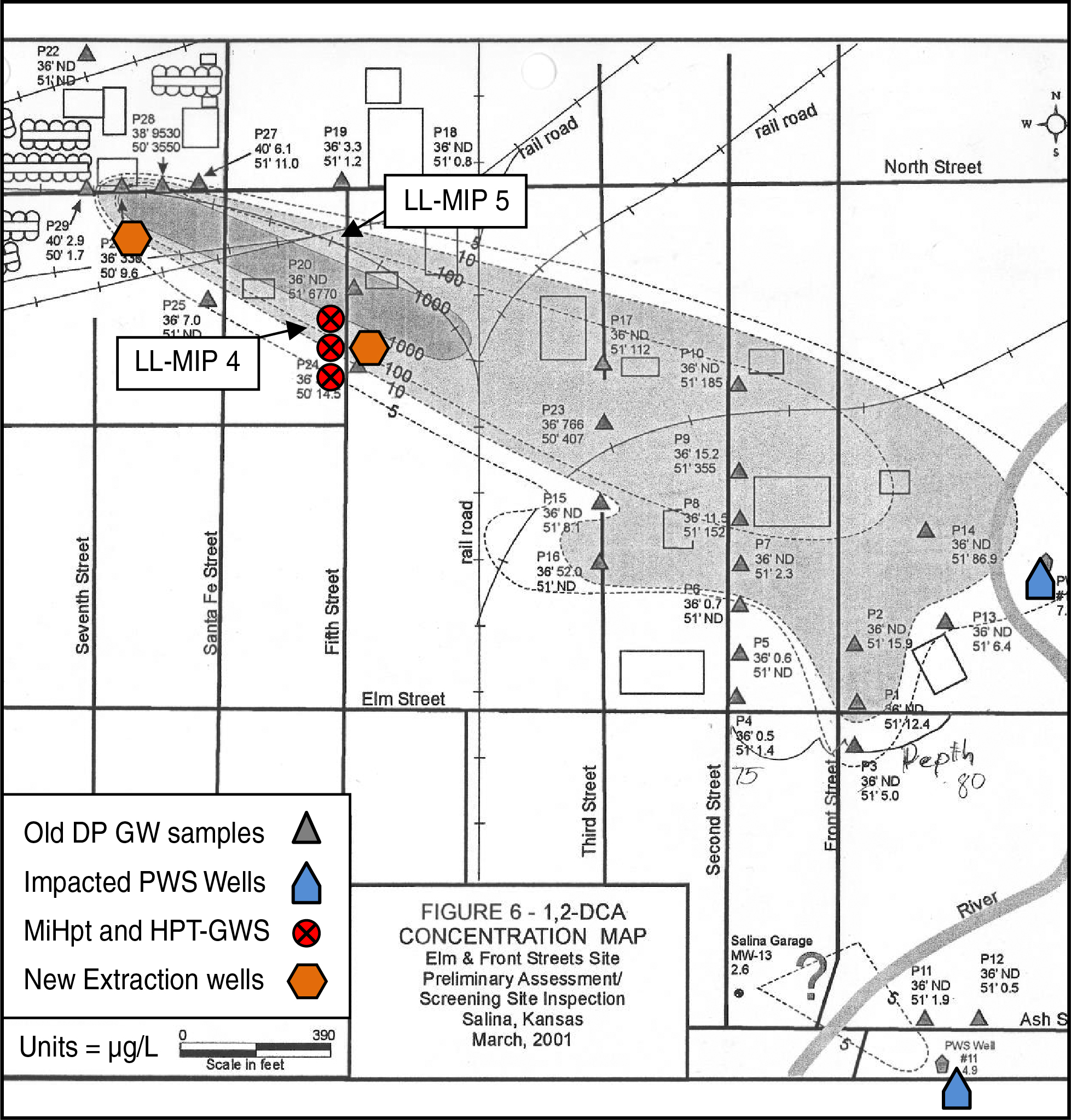
Figure G-14. Site map.
The log shown in Figure G-15 is the one in the center of the short three-log transect depicted in Figure G-14. From the surface to a depth of about 30 ft below grade, both the EC log (left) and HPT pressure log (center) are relatively high, indicating a large amount of clay and silt in the formation with relatively low permeability. Where the EC and HPT are lower (~7 ft–4 ft), there is an increase in the silt and sand content in the formation. Below 30 ft, the EC is generally below 50 millisiemens per meter, indicating mostly sand and gravel. The peaks and spikes in EC across this zone suggest an increase in clay content (clay lenses), and it is evident that the HPT pressure increases over most of these same intervals, indicating lower permeability. The right graph provides the log of the XSD detector. The XSD is sensitive to X-VOCs; thus, the presence of X-VOCs in the formation is evident by the elevated responses over the two zones in the log.
The red triangles on the HPT pressure log mark the depths at which the probe advancement was stopped, the HPT injection flow turned off, and dissipation test run to determine the local hydrostatic pressure. The blue dashed line below 30 ft indicates the piezometric pressure line, showing how the water pressure increases below the static water level. The black circle just above 30 ft represents the calculated water level based on the dissipation test results.

Figure G-15. EC log left, HPT log center, and XSD log right.
Figure G-16 illustrates the same log as Figure G-15, but with the XSD detector log replaced by the corrected HPT pressure (right graph). The corrected HPT pressure log is obtained by subtracting the atmospheric pressure and piezometric pressure from the HPT pressure log at each depth interval. The corrected HPT pressure shows the actual pressure required to inject water into the formation, without the atmospheric and piezometric pressure influences. Thus, the pressure required to inject water into the formation at 34 ft, 44 ft, and 54 ft is approximately equal in this formation, as is the permeability at the three depth intervals.
The inset box below displays the dissipation test run at the 56.72 ft depth, along with the stabilized piezometric pressure for that depth.

Figure G-16. Corrected HPT Log from Figure G-15.
Figure G-17 is a simple cross section of the three logs obtained across the plume. The logs were run about 30ft apart in an N-S transect. The corrected HPT pressure is depicted by the solid purple line and the EC is depicted by the dashed black line. The EC and HPT pressure measure two different physical parameters of the soil–bulk EC of the formation and permeability, respectively. The EC responds primarily to the clay content of this formation. At this site, the clay content and the HPT pressure correlate well, indicating that clay content is the primary influence on formation permeability. In general, as the EC increases, the HPT pressure increases and vice-versa. This cross section shows that the upper 30 ft of the formation is primarily fine-grained material with low to moderate permeability at best and that, below 30 ft, the formation is primarily sand and gravel with lenses of clay (higher EC and HPT pressure). The clay-rich layer at depths of approximately 36 ft–40 ft (between dot-dash lines) appears to be continuous across the area logged; however, the clay content appears to be lower and the permeability higher at the center log (N425) than at the other two locations.

Figure G-17. Cross section of the three MiHpt logs showing corrected HPT pressure and EC (dashed).
In Figure G-18, the XSD response (solid red line) is laid over the EC log (black dash with gray fill). These logs were obtained with the low-level MiHpt system, which provides lower detection limits (about 10X) so that lower concentrations of X-VOCs at the edge of the plume are detectable. The horizontal scales for EC and XSD are the same for each log, so the magnitude of the XSD response is consistent across the logs. The core of the plume is to the north (log N-5A) and the edge of the plume is to the south (log N-4). This is apparent as the magnitude of the XSD response decreases from north to south along the transect. In the core of the plume (log N-5A), the X-VOC contamination is generally dispersed across the sandy aquifer materials. There is an upper zone (~38 ft–45 ft) and lower zone (~48 ft–57 ft) at which detector response is high, with a decrease in response between these zones. Moving south away from the core of the plume, the XSD response (and thus X-VOC concentrations) are focused around some of the clay lenses (dashed ovals). It therefore appears that, as the plume ages and remediation progresses, X-VOC contaminants in the sandy aquifer materials are removed while those sorbed into the clay lenses remain. Further, the relationship between the clay lenses defined by the EC logs and the surrounding XSD response indicates that the contaminated clay lenses are behaving as a low-permeability source, slowly feeding X-VOCs back into the sandy aquifer materials around the clay lenses.

Figure G-18. Cross section with EC and XSD response indicating back-diffusion from clay lenses.
The Figure G-19 cross section, with corrected HPT pressure and XSD detector response, suggests the same relationship between the lower-permeability (higher HPT pressure) clay lenses and the X-VOC contamination as that observed in Figure G-18. South of the plume core, the clay lenses behave as low-permeability sources, bleeding X-VOCs back into the surrounding sandy aquifer materials.
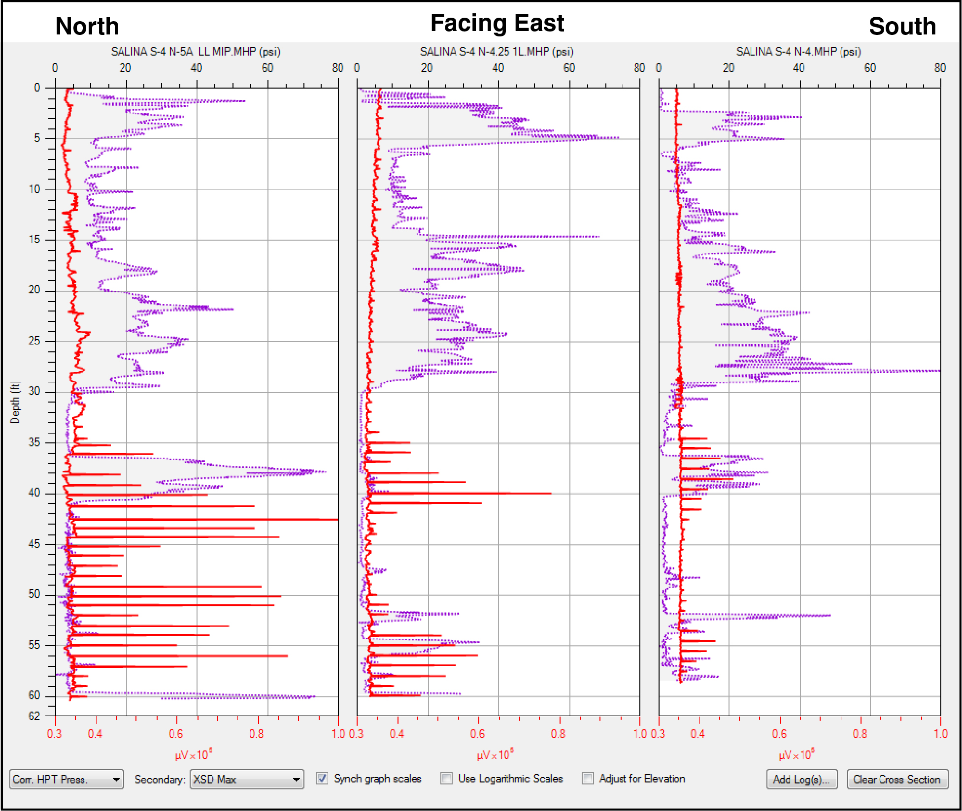
Figure G-19. Cross section with corrected HPT pressure and XSD response.
Once the low-level MiHpt logs were completed and reviewed, depth intervals were selected for groundwater profiling with the HPT-GWS system. Depths for groundwater sampling were selected based on the XSD detector response and HPT pressure. The HPT-GWS probe has four screened ports over a 4 inch vertical interval along the side of the probe. This provides for discrete interval samples. Groundwater samples cannot be collected from the high-pressure/low-permeability clay lenses, but can be obtained from the lower-pressure/higher-permeability sandy aquifer materials. Figure G-20 illustrates the HPT pressure and EC log in the left graph for the N‑5A log. The other three graphs are repeats of the XSD detector response for this log with plots of the 1,2-DCA, CCl4, and chloroform concentrations from the groundwater samples collected next to the log location. This plot shows that 1,2-DCA is the primary contaminant in the upper zone (~38 ft–45 ft) while CCl4 and its degradation product chloroform are the primary contaminants in the lower zone (~48 ft–57 ft) at this location.
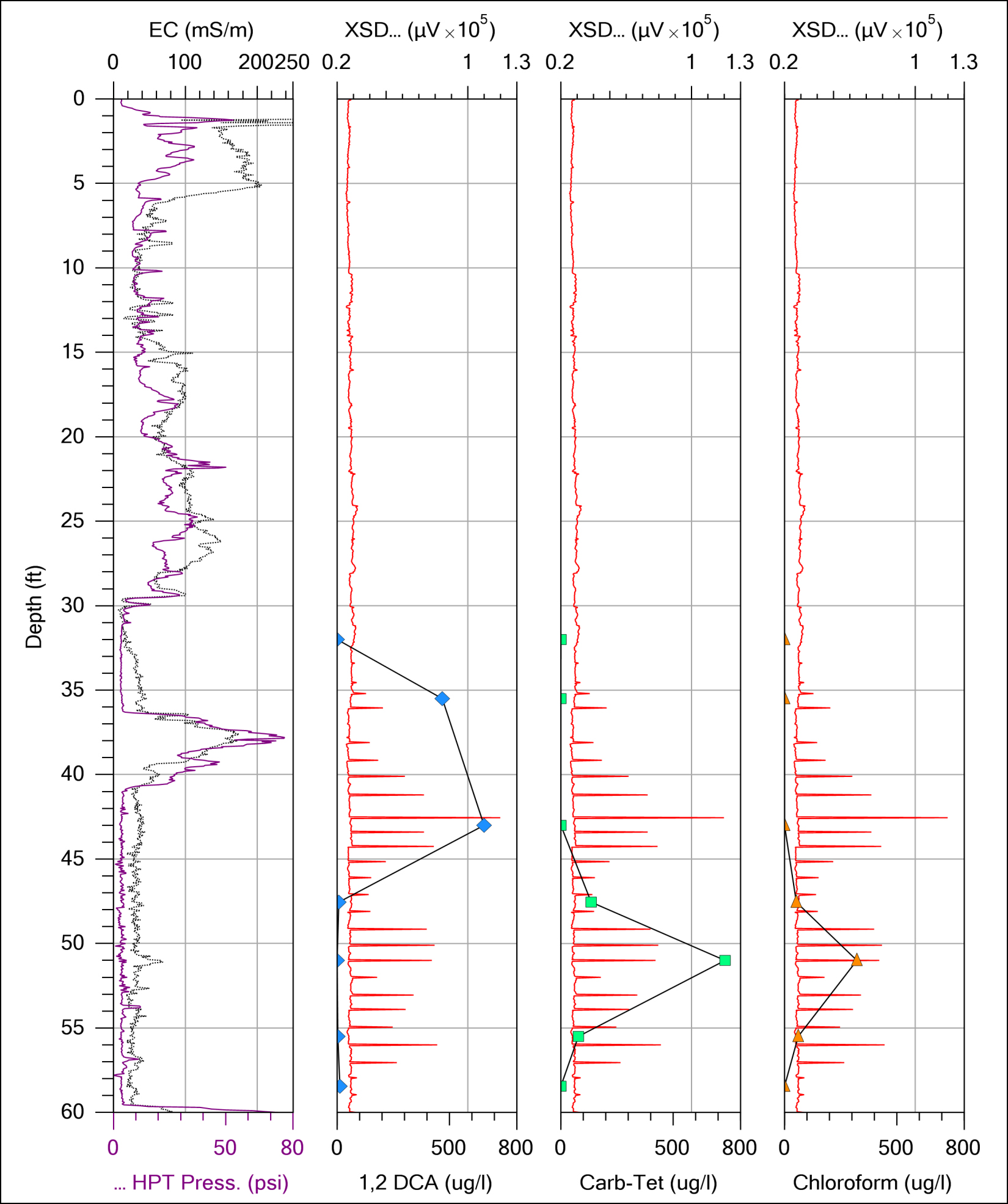
Figure G-20. The N-5A log with plots of 1,2-DCA (blue diamonds), CCl4 (green squares), and chloroform (orange triangles) plotted over the XSD log. Note that 1,2-DCA dominates in the upper zone while CCl4 and chloroform dominate in the lower zone, as defined by the XSD detector response.
Logs for the N425 and N4 locations are shown on Figure G-21, with the groundwater sample results plotted over the XSD detector response. As above, the blue diamonds represent 1,2-DCA, the green squares represent CCl4, and the orange triangles represent chloroform. Again, 1,2-DCA dominates in the upper zone while CCl4 and chloroform dominate in the lower zone, as defined by the XSD detector response.
The horizontal axes for contaminant concentration varies on these logs so that lower concentrations near the edge of the plume can be viewed at a useable scale.
On the N4 log, a sample interval at 55 ft was missed, leaving a gap in the data for this log.
For all three logs, where groundwater samples show total X-VOC concentrations increasing, the XSD detector response generally increases and vice-versa.

Figure G-21. Groundwater sample results plotted over XSD detector responses.
Figure G-22 shows all of the groundwater analyte results plotted over the N-5A XSD detector log. This more clearly defines the upper zone with 1,2-DCA, while the lower zone consists mostly of CCl4 and its primary degradation product chloroform. The MIP XSD detector response provides a clear indication of total X-VOC contaminant load vs. depth, but not specificity; however, the groundwater profile samples provide the specificity (analyte ID) necessary for discerning the contaminant zones.
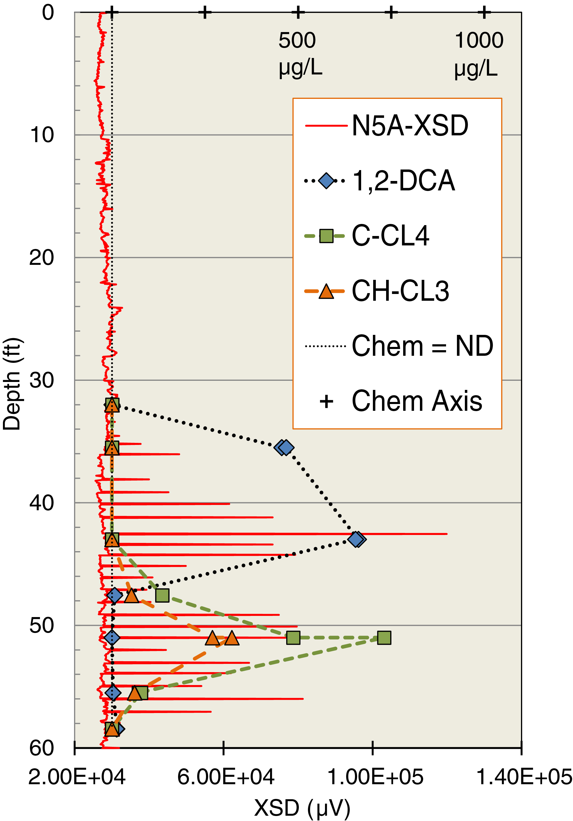
Figure G-22. Groundwater analyte results plotted over XSD detector log.
With the groundwater profile sample results, Figure G-23 shows the distribution of the contaminants in the subsurface. There is an upper groundwater plume consisting primarily of 1,2-DCA (dashed line with orange fill) and a deeper groundwater plume consisting primarily of CCl4 and chlo
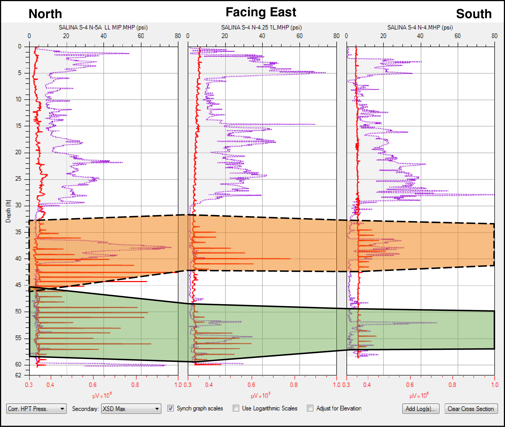
Figure G-23. Cross section with corrected HPT pressure and XSD response.